이번에는 Tensorflow 튜토리얼 예제중에서 매카니즘을 살펴보도록 하겠습니다.
이번 예제는 총 3개의 Layer로 구성되어 있는 Neural Network 기반의 예제입니다.
여기서는 NN을 구현하는 목적에 관련된 것이라니 보다는 Tensorflow를 활용해서 구현을 할때 어떤 방법으로 사용되면 좋은지에 대하여 살펴볼 수 있는 예제인 것 같습니다.
더불어 TensorBoard를 이용해서 그래프를 시각적으로 볼 수 있는 내용등이 포함되어 있습니다.
튜토리얼을 텐서플로 코리아에서 환글화를 해주셔서 편하게 한번 읽어 볼 수 있고, 해당 예제 소스도 다운로드 받을 수 있으니 한번씩 보시면 좋을 것 같습니다.
<TensorFlow Mechanics 101 한글화 문서 바로라기>
먼저 소스를 내려받아서 실행을 해보면 다음과 같이 콘솔상에 결과 화면을 볼 수 있습니다.
Extracting data/train-images-idx3-ubyte.gz
Extracting data/train-labels-idx1-ubyte.gz
Extracting data/t10k-images-idx3-ubyte.gz
Extracting data/t10k-labels-idx1-ubyte.gz
Step 0: loss = 2.32 (0.009 sec)
Step 100: loss = 2.15 (0.004 sec)
Step 1500: loss = 0.35 (0.004 sec)
Step 1600: loss = 0.36 (0.004 sec)
Step 1700: loss = 0.48 (0.005 sec)
Step 1800: loss = 0.33 (0.005 sec)
Step 1900: loss = 0.45 (0.005 sec)
Training Data Eval:
data_set.num_examples: 55000 FLAGS.batch_size: 100 steps_per_epoch:550.000000
Num examples: 55000 Num correct: 49240 Precision @ 1: 0.8953
Validation Data Eval:
data_set.num_examples: 5000 FLAGS.batch_size: 100 steps_per_epoch:50.000000
Num examples: 5000 Num correct: 4519 Precision @ 1: 0.9038
Test Data Eval:
data_set.num_examples: 10000 FLAGS.batch_size: 100 steps_per_epoch:100.000000
Num examples: 10000 Num correct: 9024 Precision @ 1: 0.9024
실행을 하게 되면 가장 먼저 MNIST의 이미지 데이터들을 다운로드 받아 옵니다.
MNIST는 28 x 28 크기를 가지는 이미지들로 구성이 되어 있습니다. 이 이미지들은 사람이 손글씨로 쓴 0~9까지의 숫자들입니다. 이 이미지 데이터를 기본으로 머신러닝의 알고리즘을 테스트하고 인식율을 측정하는데 많이 사용되는 이미지 데이터셋입니다.
(http://yann.lecun.com/exdb/mnist/)
이 이미지들을 학습하여 약 90%의 정확성을 보이는 결과를 볼 수 있습니다.
그러면 이제 튜토리얼도 한번 읽어보고 실행도 한번 해보았으니 소스를 간단하게 살펴보도록 하겠습니다.
이 예제의 시작은 run_training() 함수부터 수행이 됩니다.
def run_training():
  """Train MNIST for a number of steps."""
  # Get the sets of images and labels for training, validation, and
  # test on MNIST.
  data_sets = input_data.read_data_sets(FLAGS.train_dir, FLAGS.fake_data)
가장 먼저 하게 되는 것은 이미지 데이터 셋을 다운로드 받아 압축을 해제합니다. 그런후 Numpy 4차원 배열로 담아 메모리에 올리고 이를 data_set 이라는 이름의 Collection 객체로 지정을 합니다.
이때 사용되는 함수들은 Tensorflow contrib 에서 기본 제공되는 것들이니 만약 여기서 오류가 발생한다면 Tensorflow 버젼을 업그레이드 해보면 될 겁니다.
이렇게 데이터를 잘 받아왔으면 다음 디폴트 Graph를 지정합니다. 명시하나 안하나 별 차이는 없지만 명시해주는 것이 좋겠지요.
# Tell TensorFlow that the model will be built into the default Graph.
with tf.Graph().as_default():
이제부터 본격적으로 Tensorflow의 Graph를 구성하기 시작합니다.
batch_size 만큼의 크기의 placeholder를 이미지와 레이블을 추가합니다.# Generate placeholders for the images and labels.
images_placeholder, labels_placeholder = placeholder_inputs(
FLAGS.batch_size)
그리고 Layer 구성을 만들어주는 mnist.inference() 함수를 호출합니다.
# Build a Graph that computes predictions from the inference model.
logits = mnist.inference(images_placeholder,
                         FLAGS.hidden1,
                         FLAGS.hidden2)
이 함수를 잠시 살펴보면,
3개의 Layer를 구성하는 것은 특별한 내용이 없지만,
각 Layer를 구성하면서 with tf.name_scope(): 구문을 사용해서 레이어 이름별로 범위를 나누어 주었습니다.
이렇게 구성을 하면 각각의 scope 내에서 동일한 이름의 변수를 사용할 수도 있고, 이 이름으로 생성된 scope는 나중에 TensorBoard에서 보다 이쁘게 구분되어 볼 수 있어 유용합니다.
def inference(images, hidden1_units, hidden2_units):
  """Build the MNIST model up to where it may be used for inference.

  Args:
    images: Images placeholder, from inputs().
    hidden1_units: Size of the first hidden layer.
    hidden2_units: Size of the second hidden layer.

  Returns:
    softmax_linear: Output tensor with the computed logits.
  """
  # Hidden 1
  with tf.name_scope('hidden1'):
    weights = tf.Variable(
        tf.truncated_normal([IMAGE_PIXELS, hidden1_units],
                            stddev=1.0 / math.sqrt(float(IMAGE_PIXELS))),
        name='weights')
    biases = tf.Variable(tf.zeros([hidden1_units]),
                         name='biases')
    hidden1 = tf.nn.relu(tf.matmul(images, weights) + biases)
  # Hidden 2
  with tf.name_scope('hidden2'):
    weights = tf.Variable(
        tf.truncated_normal([hidden1_units, hidden2_units],
                            stddev=1.0 / math.sqrt(float(hidden1_units))),
        name='weights')
    biases = tf.Variable(tf.zeros([hidden2_units]),
                         name='biases')
    hidden2 = tf.nn.relu(tf.matmul(hidden1, weights) + biases)
  # Linear
  with tf.name_scope('softmax_linear'):
    weights = tf.Variable(
        tf.truncated_normal([hidden2_units, NUM_CLASSES],
                            stddev=1.0 / math.sqrt(float(hidden2_units))),
        name='weights')
    biases = tf.Variable(tf.zeros([NUM_CLASSES]),
                         name='biases')
    logits = tf.matmul(hidden2, weights) + biases
  return logits
이렇게 하여 기본적인 학습 모델이 Graph에 추가가 되었습니다.
그런 다음에 loss를 측정하기 위한 mnist.loss() 함수를 호출하고,
Gradient Descent 알고리즘으로 Training을 하기 위한 mnist.training() 함수를 호출합니다.
그리고 결과를 평가하기 위한 mnist.evaluation() 함수를 호출하여 Graph를 구성하게 됩니다.
# Add to the Graph the Ops for loss calculation.
loss = mnist.loss(logits, labels_placeholder)

# Add to the Graph the Ops that calculate and apply gradients.
train_op = mnist.training(loss, FLAGS.learning_rate)

# Add the Op to compare the logits to the labels during evaluation.
eval_correct = mnist.evaluation(logits, labels_placeholder)
이제부터는 부가적인 기능을 위하여 TensorBoard와 데이터 파일 저장, 그리고 세션을 준비하게 됩니다.
앞의 포스팅에서 TensorBoard를 간단하게 알아보았는데 여기서 활용을 합니다.
summary를 생성하여 TensorBoard를 준비하고,
모든 변수들을 초기화 하기 위한 init을 추가하고,
파일 저장 및 로딩을 위한 saver를 추가하고,
Session을 생성합니다.
그리고 TensorBoard를 위한 데이터 저장할 디렉토리와 생성된 Session 정보를 통해서 summary_writer 객체를 생성합니다.
최종적으로 init 을 세션에서 한번 실행해줘서 변수들을 초기화 해주면, 이제 실제 실행을 하기 위한 기본적인 준비가 완료되었습니다.
# Build the summary Tensor based on the TF collection of Summaries.
summary = tf.merge_all_summaries()

# Add the variable initializer Op.
init = tf.initialize_all_variables()

# Create a saver for writing training checkpoints.
saver = tf.train.Saver()

# Create a session for running Ops on the Graph.
sess = tf.Session()

# Instantiate a SummaryWriter to output summaries and the Graph.
summary_writer = tf.train.SummaryWriter(FLAGS.train_dir, sess.graph)

# And then after everything is built:

# Run the Op to initialize the variables.
sess.run(init)
세션내에서 실행을 하기 위해서 loop를 batch_size 만큼 돌려줍니다.
xrange는 library를 사용한 것인데 0부터 FLAGS.max_steps 만큼 반복적으로 내부의 로직들을 수행하게 됩니다.
train 이미지 데이터들 feed_dict에 담고,
sess.run() 으로 알고리즘 모델과 loss를 실행합니다.
# Start the training loop.
for step in xrange(FLAGS.max_steps):
  start_time = time.time()

  # Fill a feed dictionary with the actual set of images and labels
  # for this particular training step.
  feed_dict = fill_feed_dict(data_sets.train,
                             images_placeholder,
                             labels_placeholder)

  # Run one step of the model.  The return values are the activations
  # from the `train_op` (which is discarded) and the `loss` Op.  To
  # inspect the values of your Ops or variables, you may include them
  # in the list passed to sess.run() and the value tensors will be
  # returned in the tuple from the call.
  _, loss_value = sess.run([train_op, loss],
                           feed_dict=feed_dict)

  duration = time.time() - start_time
반복문이 100번 돌때 1번 실행하면서,
콘솔에 print를 하고 summary_writer 의 add_summary() 함수를 통해서 TensorBoard에 그래프로 데이터를 표현하기 위한 로깅을 하게 되어 있습니다.
# Write the summaries and print an overview fairly often.
if step % 100 == 0:
  # Print status to stdout.
  print('Step %d: loss = %.2f (%.3f sec)' % (step, loss_value, duration))
  # Update the events file.
  summary_str = sess.run(summary, feed_dict=feed_dict)
  summary_writer.add_summary(summary_str, step)
  summary_writer.flush()
이제 마지막으로 1000번에 한번씩 혹은 마지막에 수행되도록 하여,
checkpoint_file을 디스크에 실제 파일로 저장하도록 해줍니다. 중간중간 이렇게 저장된 파일의 데이터는 다시 로딩을 하거나 학습한 중간 결과를 저장하는데 유용하게 사용할 수 있습니다.
그리고 현재까지의 학습에 따른 train 셋과 Validation 셋과 Test 셋의 전체 데이터를 이용해서 정확도를 체크하는 함수를 한번씩 수행합니다.
# Save a checkpoint and evaluate the model periodically.
if (step + 1) % 1000 == 0 or (step + 1) == FLAGS.max_steps:
  checkpoint_file = os.path.join(FLAGS.train_dir, 'checkpoint')
  saver.save(sess, checkpoint_file, global_step=step)
  # Evaluate against the training set.
  print('Training Data Eval:')
  do_eval(sess,
          eval_correct,
          images_placeholder,
          labels_placeholder,
          data_sets.train)
  # Evaluate against the validation set.
  print('Validation Data Eval:')
  do_eval(sess,
          eval_correct,
          images_placeholder,
          labels_placeholder,
          data_sets.validation)
  # Evaluate against the test set.
  print('Test Data Eval:')
  do_eval(sess,
          eval_correct,
          images_placeholder,
          labels_placeholder,
          data_sets.test)
이렇게 하여 최종 실행이 완료되면, 서버의 ./data 디렉토리가 생성이 되고 파일 데이터들이 생성이 됩니다.
콘솔에서 아래와 같이 TensorBoard를 구동하고, 웹브라우저에서 6006 포트로 접속을 해보면,
$ TensorBoard --logdir=.
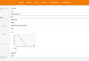
아래와 같이 TensorBoard를 통해서 데이터 그래프와 Tensorflow Graph 모델을 볼 수 있습니다.
이 Graph는 우리가 지정해준 scope가 박스로 표현이 되고 해당 박스의 오른쪽을 클릭하여 상세내용을 펼쳐 볼수도 있습니다.


이로서 기본적인 Tensorflow의 매카니즘을 살펴보았습니다.
'Tensorflow' 카테고리의 다른 글
| 14. Tensorflow 시작하기 - Wide & Deep Learning (0) | 2016.11.08 |
|---|---|
| 13. Tensorflow 시작하기 - tf.contrib.learn Quickstart (2) | 2016.11.07 |
| 11. Tensorflow 시작하기 - TensorBoard (0) | 2016.11.05 |
| 10. Tensorflow 시작하기 - flags (3) | 2016.11.04 |
| 9. Tensorflow 시작하기 - Session (2) | 2016.10.25 |


댓글